HexagonDiff

HexagonDiff is a Python tool for differential verification of deep neural networks (DNNs) on Hexagon DSPs. It compares the outputs of two DNN implementations to identify discrepancies and ensure correctness.

Command-line Usage

To use HexagonDiff, run the following command in your terminal:

Usage: hexagon_diff [options] <nn1> <nn2> <spec>

    <nn1> and <nn2> are the paths to the two DNN implementations to be compared (ONNX format).
    <spec> is the input specification file (VNNLIB).


Options:
  --epsilon EPSILON     Verify Epsilon Equivalence (L-infinity norm); provides the epsilon value (type: Float64, default: -Inf)
  --top-1               Verify Top-1 Equivalence
  --timeout TIMEOUT     Timeout for verification (type: Int64, default: 0)
  -h, --help            Show this help message and exit
  -v, --verbose         Enable verbose output for detailed comparison results

Note that one single VNNLIB specification file is used for both DNNs, and the specification must be in the form of $\mathbf{lb}\le \mathbf{x}\le \mathbf{ub}$, where $\mathbf{lb}$ and $\mathbf{ub}$ are the lower and upper bounds of the input, respectively. Examples are available in the examples directory.

Dependencies

HexagonDiff relies on the following libraries:

• onnx: For parsing ONNX models.
• torch: For linear algebra operations and auto differentiation.
• triton: For GPU acceleration of verification code.

Preprocessing (A prompt to AI Code Generation)

HexagonDiff is a C++ tool for differential verification of deep neural networks (DNNs) on Hexagon DSPs. It compares the outputs of two DNN implementations to identify discrepancies and ensure correctness.

Basics

Use onnx library to parse the ONNX models of the two DNN implementations. Extract the computational graph, input/output tensors, and parameters for each layer.

Write your own parser to read the VNNLIB specification file. Assume that the input specifications are in the form of $\mathbf{lb}\le \mathbf{x}\le \mathbf{ub}$, where $\mathbf{lb}$ and $\mathbf{ub}$ are the lower and upper bounds of the input, respectively.

Write most of your operation in torch. For operations doesn't exist in torch, write your own implementation using triton for GPU acceleration.

Differential Network

We assume that two DNN implementations are only different in certain layers, such as affine layers and token pruning layers, which means we can construct a differential network. The differential network has the same structure as the original network, except the following differences:

1. All non-linear operators (e.g., ReLU, MaxPool) remained the same as in the original two DNNs.
2. If the two networks have different weight and bias in a certain affine layer, in the differential network, we keep weights and biases from both the DNNs: $(W_x,W_y,b_x,b_y)$ as the affine operator in the differential network.
3. We denote each edge of the network as different types of tensors. During the verification of the network, these different type will be bounded differently. At the current stage, we only consider the following types of tensors:
   1. $\mathrm{Eq}(\mathbf{x},\mathbf{y})$ represents that the two DNNs have the exact same value at this point. Later, we will bound $\mathbf{x}$ and $\mathbf{y}$ using the same bounds: $\mathbf{lb}\le \mathbf{x},\mathbf{y}\le \mathbf{ub}$.
   2. $\mathrm{Diff}(\mathbf{x},\mathbf{y})$ represents that the two DNNs have different values but same shape at this point. Later, we will bound $\mathbf{x}$ and $\mathbf{y}$ separately: ${\mathbf{lb}}_x\le \mathbf{x}\le {\mathbf{ub}}_x$ and ${\mathbf{lb}}_y\le \mathbf{y}\le {\mathbf{ub}}_y$, and with a differential bound: ${\mathbf{lb}}_d\le \mathbf{y}-\mathbf{\beta }\mathbf{x}\le {\mathbf{ub}}_d,\mathbf{\beta }=\frac{\mathbf{uy}-\mathbf{ly}}{\mathbf{ux}-\mathbf{lx}}$.
   3. $\mathrm{Truncate}(\mathbf{x},\mathbf{y})$ represents that the one vector (tensor) of the differential network is truncated from the other. Later, we will bound the common part of $\mathbf{x}$ and $\mathbf{y}$ using the same bounds as $\mathrm{Diff}$, and bound the truncated part of $\mathbf{y}$ using a single bound of $\mathbf{y}$: ${\mathbf{lb}}_y\le \mathbf{y}\le {\mathbf{ub}}_y$.
   4. $\mathrm{TruncateMerge}(\mathbf{x},\mathbf{y})$ represents that the one vector (tensor) of the differential network is truncated from the other, and the truncated part is merged into the last vector (tensor). In addition to $\mathrm{Truncate}$, we also need to bound the $\mathrm{Diff}$ bounds between every value (tensor) in the truncated part and the merged value (tensor). For example, if vector $\mathbf{y}$ is truncated from vector $\mathbf{x}$, we need to bound $\mathbf{x}$ and $\mathbf{y}$ using $\mathrm{Truncate}$ bounds, and bound the difference between the last element of $\mathbf{y}$ and every element in the truncated part of $\mathbf{x}$ using $\mathrm{Diff}$ bounds.
4. For token pruning of transformers, we use special operators like $\text{TopK}$ and $\text{EViT}$ to represent the token pruning operations, which generates $\mathrm{Truncate}$ and $\mathrm{TruncateMerge}$ types.

Conversion to the Differential Network

The following changes has to be made to convert the original two DNNs into the differential network:

• LayerNorm's division needs to be removed, since this part will be difficult for verification.
• Integer tensor operations need to be fused into operators like $\text{TopK}$ and $\text{EViT}$, which will generate $\mathrm{Truncate}$ and $\mathrm{TruncateMerge}$ types.

After making these changes, we can construct the differential network by merging the two DNNs together. The two DNNs will share the same non-linear operators, and have different weights and biases for affine layers. The types in the differential network are then deduced based on the structure of the network and the differences between the two DNNs.

Verification Methods

HexagonDiff verifies the differential network using two interrelated process: linearization and bound propagation. The linearization process computes the linear dependent bounds (dbound) for each non-linear operator, which are used to approximate the non-linear operator with linear constraints. Linear dependent bounds for a 1-input 1-output operator is in the following form:

$$\begin{array}{c}{\mathbf{l}}_{\mathbf{x}}\odot \mathbf{x}+{\mathbf{lb}}_x\le f(\mathbf{x})\le {\mathbf{u}}_{\mathbf{x}}\odot \mathbf{x}+{\mathbf{ub}}_x\\ {\mathbf{l}}_{\mathbf{y}}\odot \mathbf{y}+{\mathbf{lb}}_y\le f(\mathbf{y})\le {\mathbf{u}}_{\mathbf{y}}\odot \mathbf{y}+{\mathbf{ub}}_y\\ {\mathbf{l}}_{\mathbf{\Delta x}}\odot \mathbf{x}+{\mathbf{l}}_{\mathbf{\Delta y}}\odot \mathbf{y}+{\mathbf{lb}}_{\Delta }\le f(\mathbf{y})-\mathbf{\alpha }\odot f(\mathbf{x})\le {\mathbf{u}}_{\mathbf{\Delta x}}\odot \mathbf{x}+{\mathbf{u}}_{\mathbf{\Delta y}}\odot \mathbf{y}+{\mathbf{ub}}_{\Delta }\end{array}$$

where vector $\mathbf{\alpha }\ge 0$ is a number obtained from linearization.

However, to obtain an accurate linear dependent bound, we need the bound restriction for the input of the non-linear operator. For simplicity of the linearization process, we remove the dependency and use global bound (gbound) to estimate the input of the non-linear operator, which is in the following form:

$$\begin{array}{c}\mathbf{lx}\le \mathbf{x}\le \mathbf{ux}\\ \mathbf{ly}\le \mathbf{y}\le \mathbf{uy}\\ \mathbf{ld}\le \mathbf{y}-\mathbf{\beta }\odot \mathbf{x}\le \mathbf{ud}\\ \mathbf{\beta }=\frac{\mathbf{uy}-\mathbf{ly}}{\mathbf{ux}-\mathbf{lx}}\ge 0\end{array}$$

To compute the global bound for the input of the non-linear operator, we propagate linear dependent bounds from the non-linear operator to the input layer. The linear dependent bounds for the non-linear operator are used to compute the global bound for its input, which is then used to compute the linear dependent bounds for the non-linear operator. This process is repeated until we reach the output layer of the differential network, where we can check the output specifications.

For more details about the linearization and bound propagation process, please refer to the following sections:

• Bound Propagation
• Linearization Methods

Equivalence Checking

We provide two kind of equivalence standards: epsilon equivalence and top-1 equivalence.

• Epsilon equivalence checks whether the output of the two DNNs are within an epsilon distance, which means $\Vert {\mathbf{y}}_1-{\mathbf{y}}_2\Vert \le ϵ$ where ${\mathbf{y}}_1$ and ${\mathbf{y}}_2$ are the outputs of the two DNNs, respectively.
• Top-1 equivalence checks whether the top-1 prediction of the two DNNs are the same, which means $\arg \max ({\mathbf{y}}_1)=\arg \max ({\mathbf{y}}_2)$ where ${\mathbf{y}}_1$ and ${\mathbf{y}}_2$ are the outputs of the two DNNs, respectively.

Bound Propagation

Bound propagation is a process to compute the global bound for the input of a non-linear operator in the differential network. The global bound is used to estimate the input of the non-linear operator, which is then used to compute the linear dependent bounds for the non-linear operator. The exact bounds for the input of the non-linear operator for each type is described in Preprocessing section.

Propagation Boundary $B$ is a set of edges in the differential network, where each edge represents a result $({\mathbf{x}}_i,{\mathbf{y}}_i)\in B$ from previous computation in the network. In the bound propagation process, each bound is represented as a linear combination of the results in the propagation boundary, which is in the following format:

$$\begin{array}{c}\cdot \le \mathbf{c}+\sum _{({\mathbf{x}}_i,{\mathbf{y}}_i)\in B}{A}_i{\mathbf{x}}_i+B_i{\mathbf{y}}_i\\ \text{ where }\cdot \text{ is something like }\pm \mathbf{x},\pm \mathbf{y}\text{ or }\pm (\mathbf{y}-\alpha \mathbf{x})\end{array}$$

The propagation process start with initial bounds of non-linear operator input, e.g., $\mathbf{x}-\mathbf{y}\le \mathbf{x}-\mathbf{y}$. At this point, the propagation boundary is $\{(\mathbf{x},\mathbf{y})\}$ as a starting point. Then we propagate the bounds backward in the topological order of the differential network, where each bound is represented as a linear combination of the results in the propagation boundary. When we reach the input layer of the differential network, we can obtain the global bound for the input of the non-linear operator.

Then we discuss our bound propagation method of 3 different cases: affine layers, non-linear layers and the input layer.

Affine Layers

If the next operator of the topological order is an affine layer, we can propagate the bound through the affine layer by substituting the output of the affine layer with its linear combination of its input. For example, if the next operator is a fully-connected layer represented as a tuple $({\mathbf{W}}_1,{\mathbf{b}}_1,{\mathbf{W}}_2,{\mathbf{b}}_2)$ where ${\mathbf{W}}_1$ and ${\mathbf{b}}_1$ are the weight and bias of the affine layer in the first DNN, and ${\mathbf{W}}_2$ and ${\mathbf{b}}_2$ are those in the second DNN, we can propagate the bound through this affine layer by substituting $\mathbf{x}$ with ${\mathbf{W}}_1\mathbf{x}+{\mathbf{b}}_1$ and $\mathbf{y}$ with ${\mathbf{W}}_2\mathbf{y}+{\mathbf{b}}_2$.

The input layers

Since the input specification is in the form of $\mathbf{lb}\le \mathbf{x}\le \mathbf{ub},\mathbf{lb}\le \mathbf{y}\le \mathbf{ub}$, we can propagate the bound through the input layer by substituting $\mathbf{x}$ and $\mathbf{y}$ with $\mathbf{lb}$ and $\mathbf{ub}$, and $\mathbf{y}$ with $\mathbf{lb}$ and $\mathbf{ub}$.

Given a bound in the form of $\cdot \le \mathbf{c}+\sum _{({\mathbf{x}}_i,{\mathbf{y}}_i)\in B}{A}_i{\mathbf{x}}_i+B_i{\mathbf{y}}_i$, where all $({\mathbf{x}}_i,{\mathbf{y}}_i)\in B$ are input layers. We obtain the global bound in the form of:

$$\begin{array}{c}\cdot \le \mathbf{c}+\sum _{({\mathbf{x}}_i,{\mathbf{y}}_i)\in B}{A}_i\odot {\mathbf{X}}_i+B_i\odot {\mathbf{Y}}_i\text{ where }\\ ({\mathbf{X}}_i{)}_{m,n}=\{\begin{array}{ll}({\mathbf{ub}}_i{)}_n& \text{if }(A_i{)}_{m,n}>0\\ ({\mathbf{lb}}_i{)}_n& \text{if }(A_i{)}_{m,n}<0\end{array}({\mathbf{Y}}_i{)}_{m,n}=\{\begin{array}{ll}({\mathbf{ub}}_i{)}_n& \text{if }(B_i{)}_{m,n}>0\\ ({\mathbf{lb}}_i{)}_n& \text{if }(B_i{)}_{m,n}<0\end{array}\end{array}$$

Non-linear Layers

If the next operator of the topological order is a non-linear layer, we can propagate the bound through the non-linear layer by substituting the output of the non-linear layer with its linear dependent bounds. For a 1-input 1-output non-linear operator, the linear dependent bounds are in the following form:

$$\begin{array}{c}{\mathbf{l}}_{\mathbf{x}}\odot \mathbf{x}+{\mathbf{lb}}_x\le f(\mathbf{x})\le {\mathbf{u}}_{\mathbf{x}}\odot \mathbf{x}+{\mathbf{ub}}_x\\ {\mathbf{l}}_{\mathbf{y}}\odot \mathbf{y}+{\mathbf{lb}}_y\le f(\mathbf{y})\le {\mathbf{u}}_{\mathbf{y}}\odot \mathbf{y}+{\mathbf{ub}}_y\\ {\mathbf{l}}_{\mathbf{\Delta x}}\odot \mathbf{x}+{\mathbf{l}}_{\mathbf{\Delta y}}\odot \mathbf{y}+{\mathbf{lb}}_{\Delta }\le f(\mathbf{y})-\mathbf{\alpha }\odot f(\mathbf{x})\le {\mathbf{u}}_{\mathbf{\Delta x}}\odot \mathbf{x}+{\mathbf{u}}_{\mathbf{\Delta y}}\odot \mathbf{y}+{\mathbf{ub}}_{\Delta }\end{array}$$

Given a bound in the form of $\cdot \le \mathbf{c}+Af(\mathbf{x})+Bf(\mathbf{y})$, we can propagate using the follow substitution:

$$(\cdot {)}_i\le {\mathbf{c}}_i+\sum _j{A}_{i,j}(p_{i,j}{\mathbf{x}}_j+q_{i,j}{\mathbf{y}}_j+a_{i,j})+\sum _j{B}_{i,j}(u_{i,j}{\mathbf{x}}_j+v_{i,j}{\mathbf{y}}_j+b_{i,j})$$

The value of $p_{i,j},q_{i,j},a_{i,j},u_{i,j},v_{i,j},b_{i,j}$ are divided into 6 cases based on $A_{i,j}$ and $B_{i,j}$, where each case is corresponding to a point in the hexagon:

Note that the result above may not be the optimal bound using linear programming, so further research can be done to find the optimal bound.

Linearization of Basic Non-linear Operators

Given a non-linear operator $f$ and a region $R$, we want to find linear constraints to approximate the non-linear operator, which is in the following form:

$${\mathbf{l}}^{\mathrm{T}}\mathbf{x}+\mathbf{lb}\le f(\mathbf{x})\le {\mathbf{u}}^{\mathrm{T}}\mathbf{x}+\mathbf{ub}\text{ for any }\mathbf{x}\in R$$

Specifically, given a gbound region $l_x \le x \le u_x, l_y \le y \le u_y, l_d \le y - 𝛽 x \le u_d$, we want to find linear constraints to approximate the non-linear operator $f(x)$, $f(y)$ and $f(x)-\alpha f(y)$ for any $x,y$ and some $\alpha$ in the gbound region.

Linearization Objective

Different strategies can be used to find the linear constraints. Here we consider the following two objectives:

1. Minimum $L_1$ norm of the bounds: ${\int }_R(\mathbf{u}-\mathbf{l}{)}^{\mathrm{T}}\mathbf{x}+(\mathbf{ub}-\mathbf{lb})\text{d}\mathbf{x}$.
2. Minimum $L_{\infty }$ norm of the bounds: $\underset{\mathbf{x}\in R}{\max }(\mathbf{u}-\mathbf{l}{)}^{\mathrm{T}}\mathbf{x}+(\mathbf{ub}-\mathbf{lb})$.

For me, the minimum $L_1$ bounds makes more sense because it minimizes the total area between the upper and lower bounds. In the overall algorithm, the bound will be used to restrict different directions, e.g., we may want the minimum and maximum values of $af(x)+bx$ in bound propagation. The minimum $L_1$ bounds have the ability to guarantee the average case.

At the same time, the minimum $L_1$ bounds are easier to compute. To do this, we need the convex (concave) envelope of the non-linear operator, which is the tightest convex (concave) function that upper (lower) bounds the non-linear operator, defined as follows:

$$\begin{array}{c}{f}^{\cup }=\sup \{g\mid g\text{ is convex and }g(\mathbf{x})\le f(\mathbf{x})\text{ for any }\mathbf{x}\in R\}\\ f^{\cap }=\inf \{g\mid g\text{ is concave and }g(\mathbf{x})\ge f(\mathbf{x})\text{ for any }\mathbf{x}\in R\}\end{array}$$

Then we have the formulas for the minimum $L_1$ bounds:

$$\begin{array}{c}\mathbf{l}=\nabla f^{\cup }({\mathbf{x}}_C)\mathbf{lb}=f^{\cup }({\mathbf{x}}_C)-\nabla f^{\cup }({\mathbf{x}}_C{)}^{\mathrm{T}}{\mathbf{x}}_C\\ \mathbf{u}=\nabla f^{\cap }({\mathbf{x}}_C)\mathbf{ub}=f^{\cap }({\mathbf{x}}_C)-\nabla f^{\cap }({\mathbf{x}}_C{)}^{\mathrm{T}}{\mathbf{x}}_C\end{array}$$

where ${\mathbf{x}}_C$ is the center of $R$.

Therefore, in the following sections, we will use the minimum $L_1$ bounds as the linearization objective, and we will compute the convex (concave) envelope of the non-linear operator to obtain the linear constraints.

See DeepPoly for more details about the minimum $L_1$ bounds.

Linearization Process

Before we go into the details of the linearization of specific non-linear operators, we first need to normalize the gbound to ensure that all bounds are tight. For example, for the gbound of $y$, we can compute the minimum and maximum values of $y$ in the gbound region, which are $\min\left(u_y, 𝛽 u_x + u_d\right)$ and $\max\left(l_x, 𝛽 l_x + l_d\right)$ , respectively. Then we can update the gbound of $y$ correspondingly.

Even after this, gbound area is still too complex for fast computation, thus we will try to further relax the gbound area to a parallelogram area. Obviously, there are 3 ways to relax the gbound area to a parallelogram area, which are 1) $l_x\le x\le u_x,l_y\le y\le u_y$, 2) $l_x \le x \le u_x, l_d \le y - 𝛽 x \le u_d$ and 3) $l_y \le y \le u_y, l_d \le y - 𝛽 x \le u_d$.

We choose the parrallelogram area based on these:

1. For $f(x)$ and $f(y)$, we will choose the parallelogram area of $l_x\le x\le u_x,l_y\le y\le u_y$.
2. For the convex envelope of $f(y)-\alpha f(x)$, we choose area 2) $l_x \le x \le u_x, l_d \le y - 𝛽 x \le u_d$.
3. For the concave envelope of $f(y)-\alpha f(x)$, we choose area 3) $l_y \le y \le u_y, l_d \le y - 𝛽 x \le u_d$.

We do this for simplicity and fast computation, since $\alpha ,\beta >0$, case 2 and case 3 are symmetric for computation. It simplifies our algorithm.

Selecting $\alpha$

The selection of $𝛼$ is important for the tightness of the bounds. Normally, we will select $𝛼$ based on the range of $f$ on gbound. We will discuss the selection of 𝛼 for each of the operators.

Linearization of ReLU

Linearization of ReLU(x)

def relu_lb(lb, ub):
    center = (lb + ub) / 2
    if center <= 0:
        return (0, 0)
    elif center >= 0:
        return (1, 0)

def relu_ub(lb, ub):
    k = (relu(ub) - relu(lb)) / (ub - lb)
    b = relu(lb) - k * lb
    return (k, b)

Selecting $\alpha$

def relu_alpha(lx, ux, ly, uy, ld, ud):
    return (relu(uy) - relu(ly)) / (relu(ux) - relu(lx))

Linearization of ReLU(y) - 𝛼 ReLU(x)

We only consider the area of lx ≤ x ≤ ux, ld ≤ y - 𝛽 x ≤ ud, we have the following formulas for the upper and lower bounds of $\mathrm{relu}(y) - 𝛼~ \mathrm{relu}(x)$:

def relu_diff_ub0(lx, ux, ld, ud):
    x = clip(0, lx, ux)
    k = (relu(x + ud) - relu(x + ld)) / (ud - ld)
    b = relu(x + ud) - relu(x) - k * ud
    return (k, b)

# Upper bound for `relu(𝛽x + d) - 𝛼 relu(x)`
def relu_diff_ub(lx, ux, ld, ud, 𝛼, 𝛽):
    k1, b1 = relu_diff_ub0(𝛽 lx, 𝛽 ux, ld, ud)
    if 𝛽 ≥ 𝛼:
        k2, b2 = (𝛽 - 𝛼) relu_ub(lx, ux)
    else:
        k2, b2 = (𝛽 - 𝛼) relu_lb(lx, ux)
    return k2, k1, b1 + b2

def point2line(x1, y1, x2, y2):
    k = (y2 - y1) / (x2 - x1)
    b = y1 - k * x1
    return (k, b)

# Lower bound for `relu(x + d) - 𝛼 relu(x)` (fixed d)
def relu_diff_lb0(lx, ux, d, 𝛼):
    fux = relu(ux + d) - 𝛼 * relu(ux)
    flx = relu(lx + d) - 𝛼 * relu(lx)
    lowk = (fux - flx) / (ux - lx)
    lowb = flx - lowk * lx
    if lowb + lowk * (-d) <= -𝛼 * relu(-d):
        return (lowk, lowb)
    x0 = (lx + ux) / 2
    if d >= 0 and x0 >= -d:
        p = max(lx, -d)
        return point2line(p, relu(p + d) - 𝛼 * relu(p), ux, relu(ux + d) - 𝛼 * relu(ux))
    elif d >= 0 and x0 <= -d:
        return (0, 0)
    elif d <= 0 and x0 <= -d:
        p = min(ux, -d)
        return point2line(p, relu(p + d) - 𝛼 * relu(p), lx, relu(lx + d) - 𝛼 * relu(lx))
    elif d <= 0 and x0 >= -d:
        return (1 - 𝛼, d)

# Lower bound for `relu(𝛽x + d) - 𝛼 relu(x)`
def relu_diff_lb(lx, ux, ld, ud, 𝛼, 𝛽):
    lx = lx * 𝛽
    ux = ux * 𝛽
    𝛼 = 𝛼 / 𝛽
    x0 = (lx + ux) / 2
    d0 = (ld + ud) / 2
    if x0 + d0 >= 0:
        # relu(x + d) - 𝛼 relu(x) ≥ relu(x + ud) + (d - ud) - 𝛼 relu(x)
        k, b = relu_diff_lb0(lx, ux, ud, 𝛼)
        return (k * 𝛽, 1, b - ud)
    else:
        # relu(x + d) - 𝛼 relu(x) ≥ relu(x + ld) - 𝛼 relu(x)
        k, b = relu_diff_lb0(lx, ux, ld, 𝛼)
        return (k * 𝛽, 0, b)

Open visualization in new tab

Linearization of Heaviside(x)

Here we simply provide the $\boxed{f}$ and $\boxed{f_{\Delta }}$ for ReLU, the bounds for ReLU can be easily derived using the formulas in Linearization of Basics Operators.

Boxed $h(x)$

def heaviside_box(a, b, l, u)
    = max(l ≤ x ≤ u){ a x + b heaviside(x) }
    = with
        point0 = clip(0, l, u)
        lamtop = (heaviside(point0) - heaviside(l)) / (point0 - l)
        lambot = (heaviside(u) - heaviside(point0)) / (u - point0)
        if a ≥ 0 and a + lambot b ≥ 0:
            a * u + b
        and if a ≤ 0 and a + lamtop b ≥ 0:
            a * point0 + b 
        and if a + lamtop b ≤ 0 and a ≤ 0:
            a * l
        and if a ≥ 0 and a + lamtop b ≤ 0:
            a * point0

Linearization of Exp(x)

Linearization of Exp(x)

def exp_lb(lb, ub):
    center = (lb + ub) / 2
    return (exp(center), exp(center) * (1 - center))

def exp_ub(lb, ub):
    k = (exp(ub) - exp(lb)) / (ub - lb)
    b = exp(lb) - k * lb
    return (k, b)

Selecting $\alpha$

def exp_alpha(lx, ux, ly, uy, ld, ud):
    return (exp(uy) - exp(ly)) / (exp(ux) - exp(lx))

Linearization of Exp(y) - 𝛼 Exp(x)

We only consider the area of lx ≤ x ≤ ux, ld ≤ y - 𝛽 x ≤ ud, we have the following formulas for the upper and lower bounds of $\mathrm{exp}(y) - 𝛼~ \mathrm{exp}(x)$:

# Upper bound for `exp(𝛽x + d) - 𝛼 exp(x)`
def exp_diff_ub(lx, ux, ld, ud, 𝛼, 𝛽):
    fudux = exp(𝛽 ux + ud) - 𝛼 exp(ux)
    fudlx = exp(𝛽 lx + ld) - 𝛼 exp(lx)
    k = (fudux - fudlx) / (ux - lx)
    b = fudlx - k * lx
    return k, 0, b

def point2line(x1, y1, x2, y2):
    k = (y2 - y1) / (x2 - x1)
    b = y1 - k * x1
    return (k, b)

# Lower bound for `relu(𝛽x + d) - 𝛼 relu(x)`
def relu_diff_lb(lx, ux, ld, ud, 𝛼, 𝛽):
    return (0,0,0) # TODO

Open visualization in new tab

x^2

Linearization of 1/x

For ReLU, we simply use the convex (concave) envelope of ReLU to compute the minimum $L_1$ bounds mentioned in Linearization Methods. The envelope of ReLU is in the following form:

Envelope of 1/x

def inv_cup(x, lb, ub):
    return 1 / x

def inv_cap(x, lb, ub):
    return ((ub - x) * inv(lb) + (x - lb) * inv(ub)) / (ub - lb)

Envelope of 1/x - 1/y

We only consider the area of lx ≤ x ≤ ux, ld ≤ x - y ≤ ud, we have the following formulas for the envelope of 1/x - 1/y:

def inv_diff(x, d):
    return 1/x - 1/(x - d)

Sigmoid

Tanh

Complex Neural Operators

Softmax

LayerNorm

Temperately ignored due to Shi et. al..

Token Pruning

In this section, we will discuss how to linearize token pruning methods, which are commonly used in transformer models to reduce the number of tokens and thus speed up inference. We will cover four popular token pruning methods: Top-K, EViT, POMT, and ToMe.

Top-K

Paper: Haurum2023

Code: topk

Overview

cls_attn = attn[:, :, 0, 1:]  # [B, H, N-1]
cls_attn = cls_attn.mean(dim=1)  # [B, N-1]
_, idx = torch.topk(cls_attn, left_tokens, dim=1, largest=True, sorted=True)  # [B, left_tokens]
index = idx.unsqueeze(-1).expand(-1, -1, C)  # [B, left_tokens, C]

non_cls = x[:, 1:]
x_others = torch.gather(non_cls, dim=1, index=index)  # [B, left_tokens, C]
x = torch.cat([x[:, 0:1], x_others], dim=1)

Scoring Method: Attention between spatial tokens and the [CLS] token.

• torch.topk: Returns the k largest elements of the given input tensor along a given dimension. The function returns a namedtuple (values, indices) where values is the k largest elements and indices is the indices of the k largest elements in the original input tensor.
• torch.gather: Gathers values along an axis specified by dim. For a 3-D tensor, if dim = 1, then for each value in the output tensor, it is equal to input[i][index[i][j][k]][k] where i, j, k are the indices of the output tensor.

Formalization for Linearization

The code above can be simplified into the following code (Python-like syntax).

def topk_pruning(X: Tensor[N+1, C], attn: Tensor[N+1, N+1], k: int) -> Tensor[k+1, C]:
    """
    Parameters:
    N: the number of non-class tokens
    C: the feature dimension
    k: the number of tokens to keep.

    Arguments:
    X: the input token sequence, with shape [N+1, C], where N is the number of non-class tokens and C is the feature dimension.
    attn: the attention map, with shape [N+1, N+1].
    k: the number of tokens to keep.
    """
    X_non_cls = X[1:]  # [N, C]
    scores = attn[0, 1:] # [N]
    X_new = sort_by_key(X_non_cls, scores, descending=True)  # [N, C]
    return torch.cat([X[0:1], X_new[:k]], dim=0)

def sort_by_key(X: Tensor[N, C], key: Tensor[N], descending: bool = False) -> Tensor[N, C]:
    sorted_indices = torch.argsort(key, dim=0, descending=descending)  # [N]
    return X[sorted_indices]  # [N, C]

For linearization, I rewrite the code above into the following code, using the heaviside function and delta1 function defined as follows.

def heaviside(x: Tensor) -> Tensor:
    return float(x > 0)

def delta1(x: Tensor) -> Tensor:
    return float(x == 0)

def sort_by_key(X: Tensor[N, C], key: Tensor[N], descending: bool = False) -> Tensor[N, C]:
    if descending:
        return [kth_largest(X, key, i) for i in range(N)]
    else:
        return [kth_smallest(X, key, i) for i in range(N)]

def kth_largest(X: Tensor[N, C], key: Tensor[N], k: int) -> Tensor[C]:
    for i in range(N):
        num_greater[i] = sum<j>(heaviside(key[j] - key[i]))

    return sum<i>(delta1(num_greater[i] - k) * X[i])

kth_largest function is interpreted as follows: for each token i, we count the number of tokens whose score is greater than the score of token i. If the number of tokens with greater score is equal to k, then token i is the k-th largest token, and we return its feature. Otherwise, we return 0.

EViT

Paper: Liang2022

Code: evit

Scoring Method: Attention between spatial tokens and the [CLS] token.

Overview

cls_attn = attn[:, :, 0, 1:]  # [B, H, N-1]
cls_attn = cls_attn.mean(dim=1)  # [B, N-1]
_, idx = torch.topk(cls_attn, left_tokens, dim=1, largest=True, sorted=True)  # [B, left_tokens]
index = idx.unsqueeze(-1).expand(-1, -1, C)  # [B, left_tokens, C]

non_cls = x[:, 1:]
x_others = torch.gather(non_cls, dim=1, index=index)  # [B, left_tokens, C]
compl = complement_idx(idx, N - 1)  # [B, N-1-left_tokens]
non_topk = torch.gather(non_cls, dim=1, index=compl.unsqueeze(-1).expand(-1, -1, C))  # [B, N-1-left_tokens, C]

non_topk_attn = torch.gather(cls_attn, dim=1, index=compl)  # [B, N-1-left_tokens]
extra_token = torch.sum(non_topk * non_topk_attn.unsqueeze(-1), dim=1, keepdim=True)  # [B, 1, C]
x = torch.cat([x[:, 0:1], x_others, extra_token], dim=1)

• torch.topk: Returns the k largest elements of the given input tensor along a given dimension. The function returns a namedtuple (values, indices) where values is the k largest elements and indices is the indices of the k largest elements in the original input tensor.
• torch.gather: Gathers values along an axis specified by dim. For a 3-D tensor, if dim = 1, then for each value in the output tensor, it is equal to input[i][index[i][j][k]][k] where i, j, k are the indices of the output tensor.

In addition to TopK method, EViT adds an extra token, which is the weighted average of the non-topk tokens, where the weight is the attention between the non-topk tokens and the [CLS] token.

Formalization for Linearization

The code above can be simplified into the following code, using similar sort_by_key as in TopK.

# N is the number of non-class tokens, C is the feature dimension, and k is the number of tokens to keep.
def topk_pruning(X: Tensor[N+1, C], attn: Tensor[N+1, N+1], k: int) -> Tensor[k+2, C]:
    X_non_cls = X[1:]  # [N, C]
    scores = attn[0, 1:] # [N]
    X_new, scores_new = sort_by_key(X_non_cls, scores, descending=True)  # [N, C]
    extra_token = sum(scores_new[i] * X_new[i] for i in range(k, N))  # [1, C]
    return torch.cat([X[0:1], X_new[:k], extra_token], dim=0)

def sort_by_key(X: Tensor[N, C], key: Tensor[N], descending: bool = False) -> (Tensor[N, C], Tensor[N]):
    sorted_indices = torch.argsort(key, dim=0, descending=descending)  # [N]
    return X[sorted_indices], key[sorted_indices]  # [N, C], [N]

For linearization, I rewrite the code above into the following code, using the heaviside function.

def heaviside(x: Tensor) -> Tensor:
    return float(x > 0)

def topk_pruning(X: Tensor[N+1, C], attn: Tensor[N+1, N+1], k: int) -> Tensor[k+2, C]:
    X_non_cls = X[1:]  # [N, C]
    scores = attn[0, 1:] # [N]
    extra_token = sum<i>(heaviside(scores[i] - scores[k]) * X_non_cls[i])  # [1, C]
    X_new = sort_by_key(X_non_cls, scores, descending=True)  # [N, C]
    return torch.cat([X[0:1], X_new[:k], extra_token], dim=0)

def sort_by_key(X: Tensor[N, C], key: Tensor[N], descending: bool = False) -> Tensor[N, C]:
    if descending:
        return [kth_largest(X, key, i) for i in range(N)]
    else:
        return [kth_smallest(X, key, i) for i in range(N)]

def kth_largest(X: Tensor[N, C], key: Tensor[N], k: int) -> Tensor[C]:
    for i in range(N):
        num_greater[i] = sum<j>(heaviside(key[j] - key[i]))

    return sum<i>(delta1(num_greater[i] - k) * X[i])

POMT: Prune One More Token

Paper: Eliopoulos2024

Code: POMT

Overview

POMT uses a combination of two metrics to determine which token to prune: attention-based metric and magnitude-based metric.

###
### metric_attn Measures how much each token is attended to by all other tokens - this is a metric to gauge token 'importance'
###
metric_attn = (
    torch.amax(softmax_attn[..., pomt_info.prefix_tokens :, pomt_info.prefix_tokens :], dim=1)
    .sum(dim=1, keepdim=True) # Sum along the 'rows' - this essentially counts how much a particular token is attended to by all other tokens
    .transpose(-2,-1) # Need to reshape into (B, ..., 1) instead of (B, 1, ...) shape
)
# ### Maximum possible value for any score = 1
metric_attn = metric_attn / torch.max(metric_attn)

###
### metric_magnitude estimates information content (magnitude of information) by summing features of V - this is a metric to gauge token 'importance'
###
metric_v = torch.softmax(
    torch.amax(v, dim=1)
    .sum(dim=-1, keepdim=True), # Sum along the # feature per head dimension
    dim=1 # Apply softmax across the sums of features for each token
)[:, pomt_info.prefix_tokens :] # Shave off special tokens, attenuate
### Maximum possible value for any score = 1

###
### Combine Importance Scores
###
metric = (metric_attn + metric_v)

Notably, POMT combines multiple heads of attention using a max operation, which is different from the mean operation used in Top-K and EViT. Thus, linearizing MAX operation is necessary for linearizing POMT.

offset = torch.tensor(
    data=[pomt_info.prefix_tokens], dtype=torch.long, device=x.device
)
similarity_indices = metric.argsort(dim=1, descending=True) + offset

### Keep highest scores
kept_indices = similarity_indices[:, :T]
discard_indices = similarity_indices[:, T:]

### Congregate the discarded tokens then take the mean of them
x_discarded = torch.gather(x, dim=1, index=discard_indices.expand(B, discard_indices.shape[1], C)).mean(dim=1, keepdim=True)

### Create pruned x'
x = torch.cat(
    (
        x[:, 0 : pomt_info.prefix_tokens, :],
        torch.gather(x, dim=1, index=kept_indices.expand(B, T, C)),
        x_discarded,
    ),
    dim=1,
)

So instead of weighted average of the non-topk tokens in EViT, POMT simply takes the mean of the non-topk tokens as the extra token.

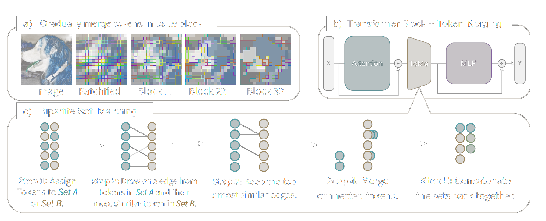
ToMe

Paper: TOKEN MERGING: YOUR VIT BUT FASTER

Code: ToMe

Overview

ToMe's attension:

B, N, C = x.shape
qkv = (
    self.qkv(x)
    .reshape(B, N, 3, self.num_heads, C // self.num_heads)
    .permute(2, 0, 3, 1, 4)
)
q, k, v = (qkv[0], qkv[1], qkv[2])

attn = (q @ k.transpose(-2, -1)) * self.scale

# Apply proportional attention (Size is the number of tokens merged into each token, used for proportional attention)
if size is not None:
    attn = attn + size.log()[:, None, None, :, 0]

attn = attn.softmax(dim=-1)
attn = self.attn_drop(attn)

x = (attn @ v).transpose(1, 2).reshape(B, N, C)
x = self.proj(x)
x = self.proj_drop(x)

# Metric is simply the mean (over multiple heads) between tokens's key.
metrics = k.mean(1)

ToMe use mean over multiple heads, similar to EViT and Top-K. Proportional attention need to be handled specially, which is not used in EViT and Top-K.

metric = metric / metric.norm(dim=-1, keepdim=True)
a, b = metric[..., ::2, :], metric[..., 1::2, :]
# Here scoring attention is computed using key from the original tokens, which is different from EViT and Top-K.
scores = a @ b.transpose(-1, -2)

if class_token:
    scores[..., 0, :] = -math.inf
if distill_token:
    scores[..., :, 0] = -math.inf

# For each node in `a`, find the node in `b` with the highest similarity score.
node_max, node_idx = scores.max(dim=-1)

# Sort the nodes in `a` based on their maximum similarity score to nodes in `b`.
edge_idx = node_max.argsort(dim=-1, descending=True)[..., None]

# Select the top `r` nodes in `a` to merge.
unm_idx = edge_idx[..., r:, :]  # Unmerged Tokens
src_idx = edge_idx[..., :r, :]  # Merged Tokens
# For each node in `a`, find the node in `b` that it is merged to.
dst_idx = node_idx[..., None].gather(dim=-2, index=src_idx)

def merge(x: torch.Tensor, mode="mean") -> torch.Tensor:
    src, dst = x[..., ::2, :], x[..., 1::2, :]
    n, t1, c = src.shape
    # Merge the tokens in `src` to the corresponding tokens in `dst` based on `dst_idx`.
    unm = src.gather(dim=-2, index=unm_idx.expand(n, t1 - r, c))
    src = src.gather(dim=-2, index=src_idx.expand(n, r, c))
    dst = dst.scatter_reduce(-2, dst_idx.expand(n, r, c), src, reduce=mode)

# Weighted average of the merged tokens, also update the size of the merged tokens
x = merge(x * size, mode="sum")
size = merge(size, mode="sum")

About Zonotopes

A special case of the linear dependent bound (dbound) formalization, where the upper and lower bounds have the same slope:

$$\begin{array}{c}{\lambda }_{\mathbf{x}}\odot \mathbf{x}+{\mathbf{lb}}_x\le f(\mathbf{x})\le {\lambda }_{\mathbf{x}}\odot \mathbf{x}+{\mathbf{ub}}_x\\ {\lambda }_{\mathbf{y}}\odot \mathbf{y}+{\mathbf{lb}}_y\le f(\mathbf{y})\le {\lambda }_{\mathbf{y}}\odot \mathbf{y}+{\mathbf{ub}}_y\\ {\lambda }_{\mathbf{\Delta x}}\odot \mathbf{x}+{\lambda }_{\mathbf{\Delta y}}\odot \mathbf{y}+{\mathbf{lb}}_{\Delta }\le f(\mathbf{x})-f(\mathbf{y})\le {\lambda }_{\mathbf{\Delta x}}\odot \mathbf{x}+{\lambda }_{\mathbf{\Delta y}}\odot \mathbf{y}+{\mathbf{ub}}_{\Delta }\end{array}$$

However, this is still not a zonotope, the area for each $(x,y)$ is a hexagon instead of a parallelogram, so to make it a zonotope, we need to further relax the hexagon area to a parallelogram area, which means we need to select one of the two slopes as the slope for both upper and lower bounds. However, there are different ways to loose this bound, it is not trivial to decide which form is better. The method proposed in Bound Propagation can be used to select the best bound, which will give a tighter bound than the standard zonotope formalization.